A Data Pipeline is a set of steps that Extract, Load and Transform data for consumption by the end user. As part of the blog series on Data Pipelines, we spoke about Data Ingestion and the different open-source and commercial players. In this blog we will talk about different data ingestion methods

The need for Data Ingestion types

In an earlier blog, we spoke about the different Data Pipeline types and how the need for data defined the data pipeline. The approaches to data ingestion we are about to explore results from the end user’s need for speed to data consumption. The Data Ingestion methods are:

  1. Batch
  2. Real-time
  3. Lambda Architecture

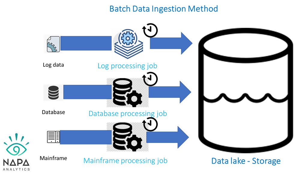
Batch Data Ingestion method

As the name suggests, the data is extracted from the source and moved to the destination at a specified time. The ingestion process could be once data or multiple times a day at a predetermined time. This method is preferred and is the most used ingestion method.

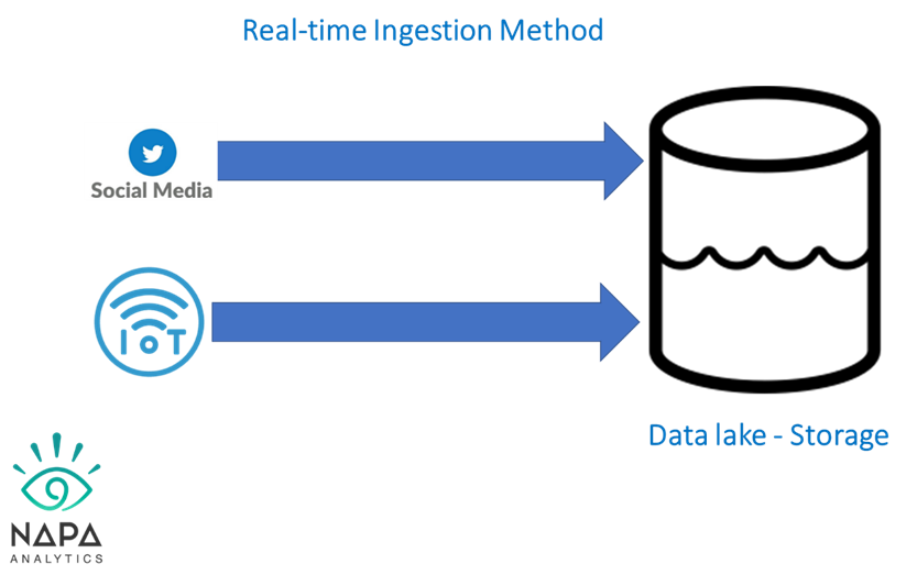
Real-time Data Ingestion Methods

Data ingestion in real-time, also known as streaming ingestion, is ongoing data ingestion from a streaming source. A streaming source can be social media feeds/listens or data from IoT devices. In this method, data retrieval and generation happen simultaneously before storage in the data lake.

Lambda architecture-based Data Ingestion Method

Lambda architecture is a data ingestion setup that consists of both real-time and batch methods. This setup consists of batch, serving, and speed layers. The first two layers index data in batches, while the speed layer instantaneously indexes the data to make it available for consumption. The presence and the activities from each layer ensure that data is available for consumption with low latency.

Summary

Data Ingestion is the first step of the ELT process and das different methods of extracting data from the sources. The data consumption needs of the data users defines the data ingestion methods as either batch, real-time, or lambda architecture. In the next blog as part of the Data Pipeline series we will talk about the Data Storage layer

In the previous blog series, we defined data pipelines, the types of data pipelines, and the data pipeline components. We identified the three main pieces of a data pipeline: Extract, Load, and Transform. In this blog, we focus on “Extract”, also referred to as Data Ingestion.

Data Ingestion

Data Ingestion is the movement of data from different data sources to a storage destination for further processing/analysis.

In the past, most of the data sources were structured making the data ingestion simple connection using JDBC/ODBC and extracting the data. With the increase in the number and variety of data sources, data ingestion has become complex. Fortunately, there are many open-source and commercial tools that take away the complexity and make it easier to extract data from a wide variety of data sources.

Data Ingestion tools

Data Ingestion tools are software products that gather and transfer structured, semi-structured, and unstructured data from the source to staging layer. The tools provide connectivity to diverse data sources, automate data movement, and monitor the movement. There are two categories of Data Ingestion tools:

  1. Open-source tools – With the increased use of Apache HDFS(Hadoop Distributed File System) is an open-source tool to store large amount of data. There are multitude of Apache open-source projects for ingesting, loading, and transforming data into HDFS and cloud storage. These tools are free to use, have a large community of developers that add to and support the feature sets.
  2. Commercial tools – These are software companies that have been in the data space and have evolved to provide the connectivity, security, UI/UX, and ease of use to ingest data from different data sources.

The figure below shows a subset of open-source and commercial solutions for data ingestion.

Prevalence of Open-source tools

Most of the ELT data pipelines use open-source tools for data ingestion. Open-source tools started to support Apache Hadoop and later Sqoop and Flume were added to extract data from structured data sources. More connectors were added as the number and variety of data sources increased. In addition, the need for real-time data led to open-source tools such as Apache Kafka, Apache Samza, Apache Nifi.

Commercial tools usage

These tools cater to users who do not have the depth of technical expertise that is required by the open-source tools. These tools provide drag-and-drop functionality and the risk management that is needed by large firms.

Which is better: open-source or commercial tools?

Commercial tools with their functionality, UI/UX, and support are welcome in most major organizations. However, open-source tools are catching up in functionality and UI/UX. Organizations are noticing the improvements in open-source tools, and the broad community support and their development teams are moving more towards open-source

Summary

Data Ingestion takes data from different data sources and loads into staging layer. There are open-source and commercial tools that are available for data ingestion. Even though commercial tools provide the support and ease of use, open-source tools are catching up and are becoming important players for Data Ingestion.

The question of ETL vs ELT is a recurring one in the world of data analytics. Historically, data engineers provide data consumers with processed data ready for consumption in a data warehouse. The process of delivering such processed data to consumers can be thoughts of as Extract, Transform, and Load (ETL). This blog demonstrated hoe data consumer needs have cause a process change to Extract, Load and Transform (ELT). Further, we explore the reasons we need to make the shift to ELT.

A large retailer and their changing data needs

Let us consider a scenario. A large retailer gets business intelligence and data analytics insights from their existing Data Warehouse. The Data Warehouse extracts information from their POS (Point of ale) and ERP (Enterprise Resource Planning) systems. The information is transformed for consumption before being loaded into the Data Warehouse. Data engineers spend a lot of time getting to consumable data hosted in the Data Warehouse. Any changes or updates would require additional analysis, development, testing, and deployment time. For data consumers, this means they would have to wait for a couple of weeks before their request for data is available for consumption.

Let us now consider that the retailer’s marketing and customer service department wants to monitor Twitter, Facebook, and other online platforms to understand the customer landscape and positive or negative chatter about the company (social listening). The data from these online platforms is not in a pre-defined format, meaning the data is in a free format and is changing all the time.

ETL to ELT transformation

Using the above example, we can review the three factors that have led to a change in thinking from Extract, Transform, and Load (ETL) to Extract, Load, and Transform ( ELT).

Data consumption requirements have changed

Our retailer must glean insights quickly from social media chatter. However, IT (Information technology) pre-defined process does not allow for consuming non-standard data formats. In addition, the velocity of data generated and data consumers (in our example, marketing and customer service department) expectations to get insights now. These change in data and demands has resulted in IT (Information Technology) to Extract and Load the data first and then worry about Transformation.

Data deluge leading to process optimization

Extraction of value at speed, from an ever-increasing volume and variety of data, requires the process to be efficient and effective, in short optimal. Social media sources have increased, and our retailer is plugged into all the different social media sources for optimal data points. The result is an increase in the variety of data sources, and an expectation to gain insights from the data sources. IT(Information Technology) takes the logical step of extract and load first and transform later

Speed of access leading to further optimization

Social media data have little shelf life, a typical social media feed loses value in a day. Data consumers, therefore, need to get access to data in near real-time. Real-time is a myth, so I am sticking to near real-time. This requirement of speed further validated the approach of Extract, Load, and Transform

Availability of Cheap Storage has accelerated the adoption of ELT

Cheap storage in form of Cloud Storage ( S3, Blob storage) is a blessing that has led to “Data Lakes” ( we will discuss this topic in our future blogs).

Summary

The confluence of the above factors has led to the shift from:

As part of the Data Pipeline series, in part one and two of the series, we talked about data pipeline and components of data pipeline. The third part deals with types of data pipelines.

The type of data pipeline is related to the need for fresh data. Data pipeline types are traditional (batch) and real-time. Data pipeline types also define the architecture and underlying technology.

Traditional (Batch) data pipeline

Traditionally, data consumption is for business intelligence and data analytics. The metrics used in business intelligence reports and analytics rely on previous data or data that was generated a few hours earlier. Thus, the data pipeline used for these consumers is a Batch Data Pipeline. As part of the batch process, data is periodically collected, loaded, and transformed at a specified time – could be once or more than once a day. Thus, the architecture and the technologies used for this data pipeline need to:

  1. Process large amounts of data
  2. Normally the batch jobs are executed when there is not much activity going on in the source system
  3. Flexibility on failures. There are options to rerun based on failure type and time allocation

Traditional Data Pipeline use case

A large retailer(with online and brick and mortar presence) has infrastructure on AWS and uses Snowflake

as their centralized data warehouse that receives data from various systems, including their online store transactional data, physical stores legacy POS system, and the web clicks from their website.

The data pipeline that caters to the web analytics team is as follows:

  1. Data from all the sources is extracted into staging tables in Snowflake
  2. Data from the staging table is loaded into the Snowflake data warehouse or to specific data marts that provide the end user behavior analytics and the features that describe the behavior
  3. Data thus aggregated is used in the analytics that is sent to the web marketing team.
Batch Processing Data Pipeline

Real time analytics

Data pipelines supporting real-time analytics provide the data and the corresponding analytics as the data is generated, like working with the stream of data called Stream processing. Stream processing is about ingesting data and calculating the metrics and analytics on every piece of data as it is generated. Real-time analytics supporting data pipelines are mainly used in places where there is lot of sensor data used to understand operations and proactively identify potential failures

Real-time data pipelines

Real-time analytics use case

A large steel manufacturing company reduced the equipment downtime by actively analyzing sensor data from the machinery. At Napa Analytics, we used the following data pipeline architecture to achieve results for our client:

  1. Text data ingested from all the machines using Kafka
  2. Data from Kafka is fed into Apache Spark for calculation and analytics
  3. Data from Apache Spark is stored in a database
  4. Messages based on thresholds are sent to distro of engineers.

Near real-time analytics

Real time analytics is not always possible. Sometimes, a compromise needs to be achieved. The compromise is what we can call near real-time analytics. In a sense, near real-time is providing data to the consumers with a time lag of 5 – 10 mins. The data pipeline structure is like the delayed (traditional data pipeline).

Near real-time use case

A large medical insurance provider has the need to look at the medical claims as they enter the system. At Napa Analytics, we used the following data pipeline architecture to achieve results for our client:

  1. Claims data from Mainframe is read into Hadoop using Apache Flume
  2. The data is loaded into Apache Kafka
  3. Processing of the data (metrics and analytics) is done using Apache Spark
  4. The output is stored in Apache Kudu
  5. The tables in Apache Kudu feed the Micro Strategy reports

From the three types of data pipelines we have examined, it is evident that data freshness is one of the deciding factors in the data pipeline you choose. If your organization needs support to select the right data pipeline suited to your needs, reach out to Contact – Napa Analytics


In our first article in the series we talked about Data Pipeline. A Data Pipeline is the process of taking data from source and getting it ready for consumption by the end users. This blog intends to explain the different data pipeline components

Data Pipeline consists of eight components as shown in the diagram below:

Data Pipeline Components

Origin

Origin is where the data is sourced from. Data can be sourced from transaction systems, social media, IoT sensors, application API’s, legacy servers, data warehouse, analytic data stores. The number of data sources and how frequently the data needs to be available for data consumers is increasing every day. Mapping data consumers expectation from the data sources is extremely important to decide the kind of data pipeline treatment given to the data from the source (Origin).

Destination

This where the data is consumed. Thus, this should be the starting point while designing a data pipeline. Data consumer requirements define the data source type, frequency, and transformation. However, the data consumer requirements also bring to light the constraints at the source (Origin). For example, in a large medical insurance company, the medical claims representative needs to see the claims as they are being generated. However, the claims processing systems takes some time (< 1 min) to move the data to the main frame system. It takes some more time for the data to move through the channel to the medical claims representative. The latency thus introduced changes the pipeline delivery SLA from real-time to near real-time. Thus, the final design needs balance data consumer requirements with the capacity and capability of Origin (Data Sources).

Dataflow

Dataflow is a set of steps that need to be orchestrated to deliver the data from Origin to Destination. Dataflow steps can sequential and/or parallel.

Parallel Dataflow
Sequential Dataflow

Dataflow steps could take the input from one step to another from Origin to Destination in a sequential manner, which is the most common Dataflow during the initial phases of Data Engineering. As the data consumption requirements mature, there is a need for an intermediate data store while maintaining the original sequential flow, this leads to the parallel data flows.

Data Storage

Data Storage is an intermediary step that enhances the data movement. There are lot of choices for an intermediate data store, and the choice needs to be based on data volume and query complexity. With the advent of new data storage options it is important to choose data storage that can support structure, format, retention duration, and is fault tolerant and has disaster recovery

Processing

This part of the data pipeline is about ingestion, persistence, transformation, and delivery. Each of the processing steps has different methods and things to consider. We will be talking about the methods and consideration in future blogs

Workflow

Workflow defines and manages the data pipeline steps. Workflow ensures that the dependencies for each of the data pipeline steps are satisfied before stating a step. Workflow needs to manage the individual steps and the overall job to achieve the results for the destination

Monitoring

Monitoring is observing the data as it moves through the data pipeline to ensure that the quality of data at the Destination.

The above components are a way to break the Data Pipeline process. Data pipeline is a key component of Data Engineering and we will talk about them in detail in the future blogs. Next Blog we will talk about the types of Data pipelines and the use cases that they support.

At Napa Analytics we take pride in helping clients with their Data Engineering needs and would love to hear from you on your Data Engineering needs/challenges. Please drop us an email at rnemani@napanalaytics.com

Data Pipeline is a sequence of steps that deliver consumable data to the end users. Why do we need a sequence of steps? In the present world, data comes from diverse sources in different formats. It is the job of a data engineer to make consumable data available to various consumers. Automated orchestration of these steps is the gist of a data pipeline.

This blog intends to talk about data pipelines. Parts of the data processes are simple, and other parts are complex. Let us start by looking at a typical data process as shown in the figure below:

Proces to deliver consumable data

The data from sources is extracted as-is and stored in the staging area. As seen from the above image, the number of data sources are finite. In the example, they are Mainframe, Cloud API, A database, and a text file. The data from the sources is stored in the staging area as one table for each source data table. Changes to the data source data structure and the addition of new data sources is not that frequent. Thus, data the data pipelines for extract and load are standard. We at Napa Analytics have built a python data framework that reduces the time and effort of creating these pipelines.

Data Pipelines

A typical data process can be considered as a combination of more than one data pipelines. The above diagram shows a typical set of data pipelines. For simplicity, we have considered only one data source (a normal situation would have more than one data sources). Dividing the data process into multiple pipelines ensures proper maintenance and ability to perform timely quality checks. Data quality is one of the main concerns with the increasing number of data sources.

Let us discuss the different pipelines:

  1. Data Pipeline # 1 – This is a straight move from Mainframe data source into staging. Staging will have a one-to-one mapping to the tables in the source database. We could go one step further of de-normalizing the data i.e., flattening the data from the multiple tables into one flat table, which can then be used to extract relevant information.
  2. Data Pipeline # 2 – 5 – These are the pipelines specific to the user requirement. For example, one of the consumers can be a MicroStrategy user who would require the table structure in a format that would feed the pre-defined reports. Another consumer can be a data analyst who is interested in dimensions and facts for aggregate analysis and reporting. Each of the consumers with their specific needs would require a specific data pipeline.

Data Pipeline(s) that deliver data in consumable format are thus a set of commands that are orchestrated to perform tasks in either sequential or parallel fashion. The initial premise of extract and load can be considered as a generic pipeline, with pipelines for transformation gaining complexity based on the consumer requirements.

The author is a data engineering expert and co-founder of Napa Analytics. Napa Analytics are working on a data framework that enables our clients with tools that reduce the effort (time and knowledge) needed in the creation and maintenance of data pipelines

Data exists in one of three states: Data at Rest, Data in Motion and Data in Use. When we understand these three states, it lays the foundation for how to extract value from that data to support business operations. This blog intends to introduce the concepts and lay a basis for the upcoming data engineering blogs in the series.

Transactional systems such as points of sale (POS), enterprise resource planning (ERP) generate and store data in a database or a mainframe. Website clicks and social media data are other sources of data. Using those two examples of types of data, we can define the three states of data.

States of Data

Data at Rest

Data at rest is data generated from a transactional system. Data analytics and business intelligence teams use data at rest to extract value. Data at rest resides in hard drives in the company’s network or cloud storage with security policies. Thus, it needs to be secure. Best practice favors encrypting data at rest and disabling access from external sources such as USB sticks or hard drives. For a long time, data at rest has been the primary source of business intelligence. Even today, dost data engineering tasks still use data at rest. The reason for the prevalence of data at rest is the existence of old systems that provide value. Another reason is that transactional systems contribute to 60% of the data sources for analytics, business intelligence, and algorithms.

Data in Motion and Data in Use

When different transactions happen in real-time, we generate Data in Motion. The shelf life of the value of data in motion is limited. To ensure the end-users get that value as soon as possible, data analytics teams need to provide data for consumption quickly. For example, social media data has mentions that have a value of maybe a day. It follows that if end users are to get any value from the data, data engineers need to extract it in less than 24 hours.

Once data is processed and available for consumption, it gives rise to Data in Use. As the name suggests, the data in use is not static or passive. And instead, it is actively moving through an IT system. Some examples of data in use include data processed in the CPU, a database or RAM.

 Now that we have identified the different data states, we will talk about extracting the data from the sources in the next set of blogs. We will also discuss how we load it into a storage layer and transform the data for consumption.